Duet3D Research – Extrusion Behaviour and Pressure Advance - Part 1
Part 1: Theory
A widespread innovation in FDM printing is the Bowden type extruder, where instead of mounting the motor that drives extrusion directly on the print head the motor is attached at a fixed location away from the print head and the filament is fed through a long flexible tube into the extruder. Bowden type extruders help to decrease the mass of the print head, which in turn allows for an increase in acceleration and/or decrease in mechanical vibrations from the printer motion system.
Bowden systems, however, have a disadvantage: The long flexible tube “softens” the response of the extruded filament, and inputs from the motor which would be relatively sharp result in a more gradual change in the rate at which material is extruded. Getting the most out of them requires software based corrections.
This is the motivation for pressure advance algorithms (also called Linear advance in some other firmwares), which apply a correction to the motor input to anticipate the “delay” in extrusion. They work by having an internal model of how the system will respond, and using this they calculate the input needed to produce the ideal output. As we will detail here, most existing implementations of pressure advance use a simple, first-order, linear model.
We showed this image at the end of our last blog post, it illustrates the predicted impact of this “delay” on 3d printed track width:
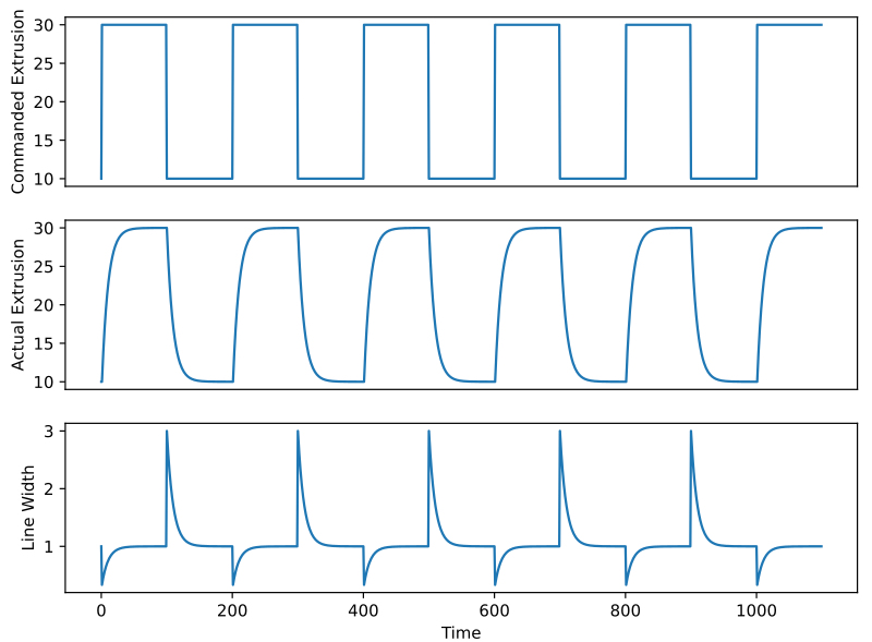 Step response from 10-30mm/s input, the expected output of the extruder and the forecast effect on line width
This post will go into the theory behind these software based corrections, and there is some maths involved, however it can be summarised as developing a formula to make the line width shown in that theoretical image as flat as possible as the speed changes.
The Pressure Advance Model
There are lots of processes in an extrusion system that contribute to the final output of a printer. Some of the most important are shown in the diagram below, which emphasises how the extruder speed and XY hot-end motion interact to determine the final track width.
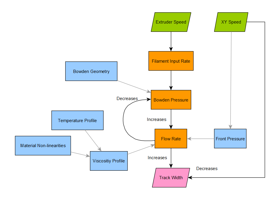 flow chart illustrating a model of an extrusion system, its inputs and outputs.
Bowden as a Spring
As filament is pushed into the Bowden tube it coils and flexes, acting like a spring. The details of this are actually quite complicated, but the standard pressure advance model uses a simple linear model: Hooke’s law, which is a standard model for a spring, and elastic behaviour more generally.
Hooke’s law relates the force exerted by a spring to its “displacement”, the distance that it is stretched or compressed. The amount of force is proportional to the displacement, and the constant of proportionality – the spring constant – determines how much.

F is the force, 𝓍 is the amount of filament in the Bowden and 𝓍eqm is the amount of filament in the Bowden at the point where there is no force, i.e. the quantity 𝓍 – 𝓍eqm is the displacement. k is the spring constant.
We can think of this as describing the “pressure” (F) inside the Bowden tube in terms of how much “extra” filament is in it (𝓍).
Relating Pressure to Feed and Extrusion Rates
Whilst the amount of extra filament in the Bowden is important, the quantities we care about measuring, such as track width, are determined by how fast the filament is extruded from the nozzle. The faster the filament comes out relative to the speed of the nozzle movement over the print surface, the narrower the width.
The difference between the rate at which filament enters the Bowden, ƒin , and output from the nozzle rate, ƒout is the amount of filament in the Bowden that changes, giving us an equation relating these quantities with the change in 𝓍.

This can then be combined with the derivative of Hooke’s law to give an equation relating the Bowden “pressure” to input and output rates.

Output Rate and Bowden “Pressure”
The last equation is all well and good, but there are two things in it we don’t know: the Bowden pressure and output rate. We need some more insight to constrain it further. To do this we can look at how the rate at which material flows out of the nozzle is connected to the Bowden “pressure”. Lots of things affect this. Some of them are shown in blue in the flowchart above. The flow of material in the nozzle is complicated, some parts are hotter or colder, and the material properties change across it. For the purposes of this model we can simplify all of this to an effective viscosity η and consider the force differential across the nozzle to be dominated by the force coming from the Bowden, giving the equation:

Along with the equation before, we can make a differential equation that describes the internal pressure (and thus output rate) of the system without reference to the amount of pressure or extra material in the system:

This equation is the model of the Bowden implicit in pressure advance corrections.
Example of the Model Behaviour
To get a feel for how this Bowden model behaves we can look at the solution for some simple values of ƒin . One particularly important case of this is a step change, which can be viewed as a transition from one constant rate input to another. This is commonly seen where the speed changes from perimeters to infill for example.
The differential equation has a well known general solution (A is a constant), details of which can be found on this Wikipedia page for those needing more information:

We can see that this describes an exponential decay of ƒout towards ƒin , asymptotically approaching ƒout = ƒin. The constant ∝ – k/η has units of Hz, and is the reciprocal of the pressure advance constant used by the Duet firmware, or, more carefully put, it is the constant used by the internal model of the extrusion behaviour which provides the basis for the pressure advance correction.
To plot this we’ll need to work out the value of A: this can be worked out from boundary conditions. Let’s calculate A for some arbitrary starting point, say, where at time t=0 the output rate is ƒout= ƒ0. This gives us an equation:

and so

and

The following is plot of this for a step change from output equilibrated to an input rate of ƒ0 to ƒin .
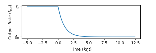 Plot of the predicted output from a step change
Input Side Corrections – Transfer Functions
The pressure advance algorithm currently used by the Duet firmware accounts for this behaviour and tries to change the input so that the output is the desired value. There is a standard way of calculating this kind of correction for many different models, including the model we have described above, using the magical powers of Laplace transforms and transfer functions.
Transfer functions are a neat way of representing the effect of a given process that is very easy to deal with mathematically. In particular, the transfer function for a sequence of (linear) processes is just the transfer function for the individual processes multiplied together.
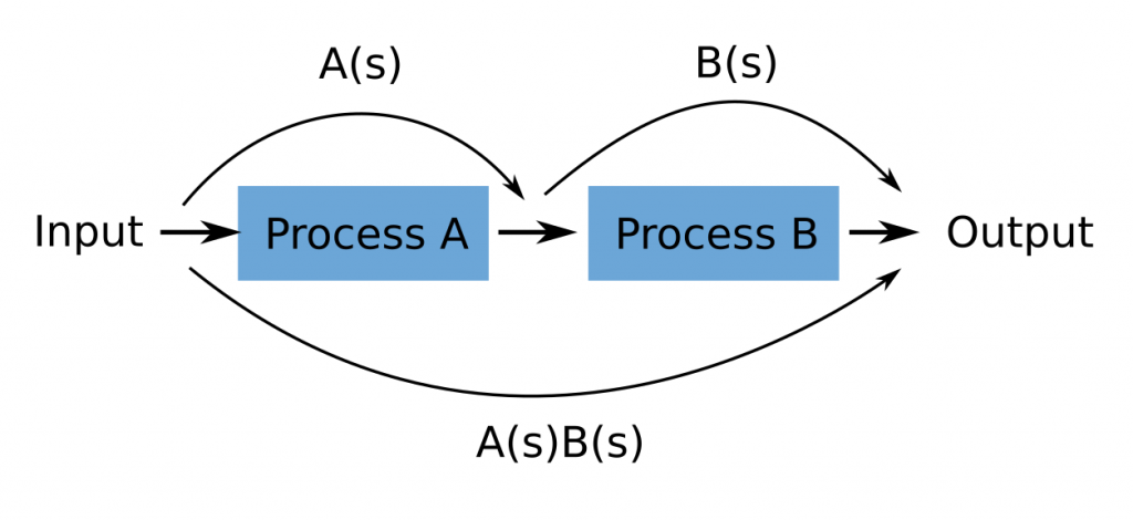 A sequence of two processes and their transfer functions, A(s) and B(s). The transfer function of the two processes in sequence combined is the product A(s)B(s).
The way that we will apply this to work out a correction is to take process B to be the Bowden, and create a process A in software that makes the output the same as input. This schema allows us to work out what the transfer function A must look like to correct for B.
Input Correcting Transfer Functions
Let’s now look at the details of the relationship between the two transfer functions above. A general transfer function, T(s), is defined as in terms of the Laplace transform, where it is the ratio of the input and output:

Here ℒ {ƒ}(s) represents the Laplace transform of ƒ, and s is the complex frequency. For the purposes here, we don’t need to worry about what s means so much, just that it is the variable over which the transfer function is defined – it is the “transformed variable” which replaces the time variable t in the original – for details see the wikipedia on the Laplace domain. For the two stage system diagrammed above this applies as follows

When A(s) is chosen correctly, we will have ƒout = ƒin , and so we have

and so

So, to work out the corrected motor input ƒ corrected we need to calculate the quantity

Where ℒ¯¹ denotes the inverse transform. In other words, we need to take the Laplace transform of our model, take its reciprocal, and transform it back.
We can now apply this to the model.
Calculating the Pressure Advance Correction
It will help to rewrite the Bowden model in terms that fit better with the scheme above. The input of the Bowden is now the corrected input ƒ corrected and for clarity we will replace η/ k with with ∝, the “pressure advance constant”.

Despite having a complicated looking definition, working with Laplace transforms is pretty easy. They add where the functions they transform add, and multiply by constants in the same way too. Where other operations are needed, Laplace transforms can just be looked at in a table, which makes applying them quite easy. Laplace transforms of derivatives are very simple too. The following is the Laplace transform for our model:

We don’t know what the Laplace transform for our input and output is ahead of time. But this doesn’t matter. Rearranging the equation above gives us the transfer function for our model, B(s):

So, as A(s) is the reciprocal of B(s):

and finally we can undo the Laplace transform to get the pressure advance correction

This describes adjusting the input velocity by adding a correction proportional to the input acceleration, and this is how the standard pressure advance algorithm is implemented. This is very simple to implement, and fast to calculate, as well as performing well in practice.
Note: The correction is very similar to a rearrangement of the equation describing the Bowden physics, but careful inspection will show that the acceleration terms are not identical (it is all in terms of ƒin ).
Theoretical Effectiveness of Pressure Advance
The pressure advance algorithm requires the model to be correct, if the model isn’t correct, the performance might not be corrected, or could even be worse. Assuming the model is correct (or at least good), it still has a constant, ⍺ , which must be matched to the system. We’ll close this part by looking at how using right and wrong values of ⍺ affect the output in the case where the model is otherwise correct.
Below is a simulation of a Bowden system with a pressure advance constant of 0.5s, reacting to transitions in speed between 15 and 30, with increasing accelerations – we will look at actual data in part 2. At this rate of change, the output without pressure advance is highly smoothed. The correction to the input increases the material pushed into the Bowden proportionally to the acceleration, meaning leading to a spiky corrected input. In this simulation the pressure advance constant used in the correction perfectly matches the constant of the Bowden.
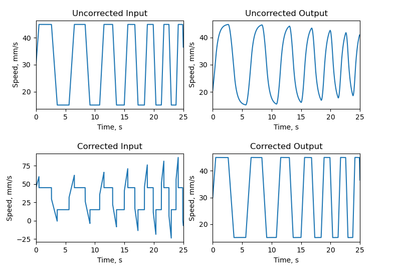 illustration of the corrections required on a step function of increasing frequency to produce an output equivalent to the input
What if we get the pressure advance constant wrong? This is shown below. In this scenario, when the pressure advance constant used in the correction is too high, it results in crests appearing on parts that should be flat, and where it is too low, there is still some remaining smoothing. The effect on width of the printed track is show also, the kind of effect on track width depends on weather the track is increasing or decreasing in size, but the direction of the effect is the same: if the PA is too high, we get over extrusion when increasing speed, and under extrusion when decreasing:
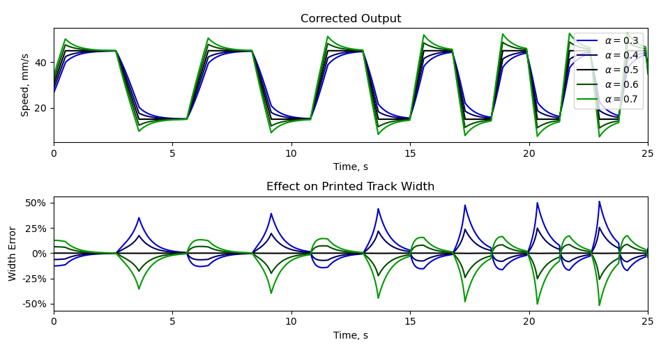 The impact of using pressure advance constants between 0.3 and 0.7 on a system where the “true” PA constant was 0.5
Coming in Part 2…
In part 2 we will look at methods we have used for estimating ⍺ using the tool changer mounted imaging system.